Click anywhere to close
OpenAI is hosting a contest to create a Sonic playing agent. The goal is to create an agent that will be able to perform well on custom hidden levels.
More information available here https://contest.openai.com/
Sonic is a very visually complex game with a parallax background, several animated foreground elements, animated enemies, and a ton of different worlds with different textures. This much noise makes it hard for an agent to gain a good understanding about the underlying game mechanics. In order to increase the signal I wanted to load in prior knowledge about the games mechanics. In Sonic it is important to have an understanding about what on screen is a solid object versus a decoration. In order to increase the signal I am giving the agent an understanding about what on screen is solid.
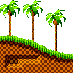
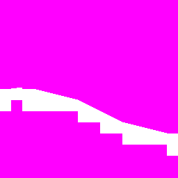
Sonic levels are built as a series of square chunks strung together to create the foreground. These chunks are place on top of a background image. Each chunk has an associated collision map that determines whether or not Sonic can pass through the pixel. The collision map will be our model’s output target.
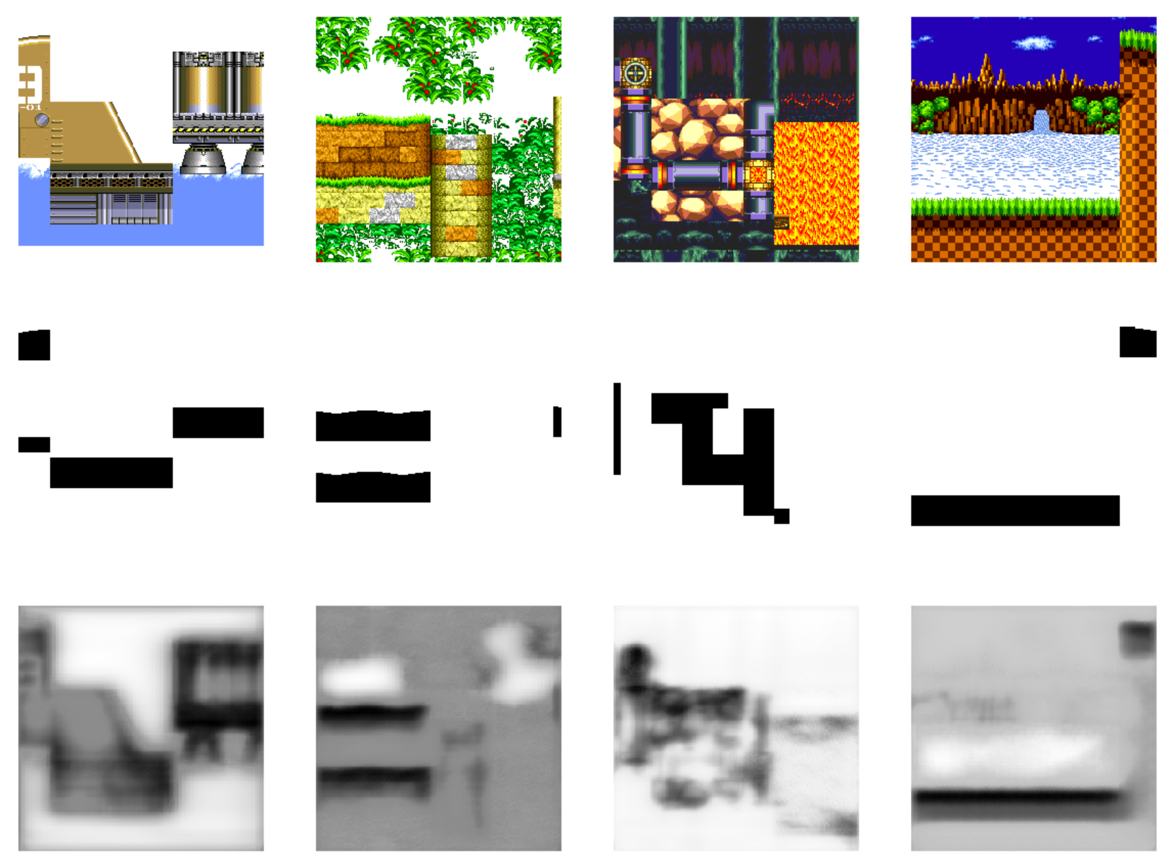
The network structure allows for any image size, so it’s up to us what size we train with. I chose 256x256 as it allows the image to contain 2-3 chunks, and the minimum height of the level backgrounds is around 256px. By randomly placing level chunks in front of a randomly offset background I am able to create tons of sample input/output.
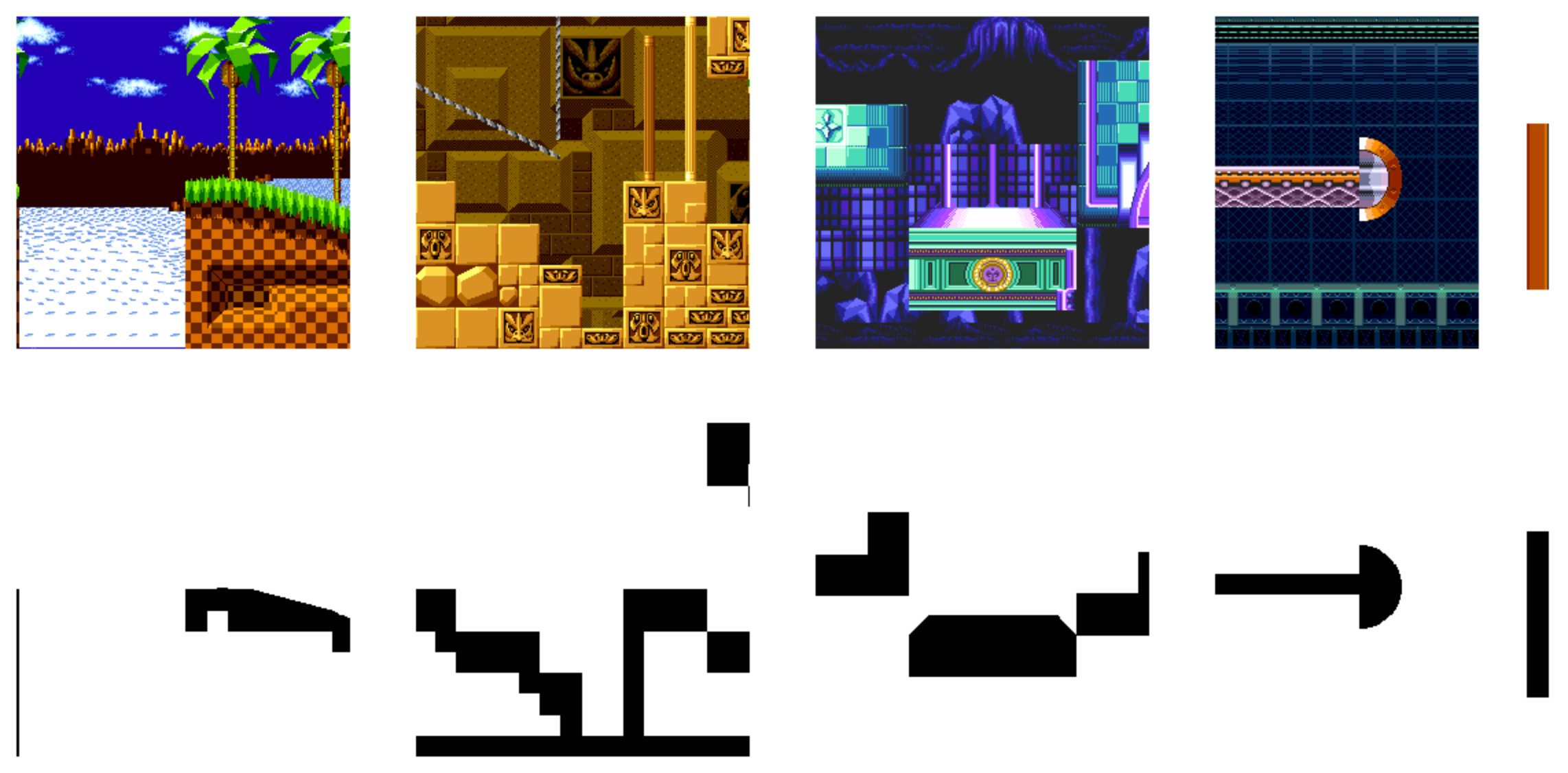
Here is an example of 4 random 256x256 images that will be used as training data (top row: input, bottom row: output target)
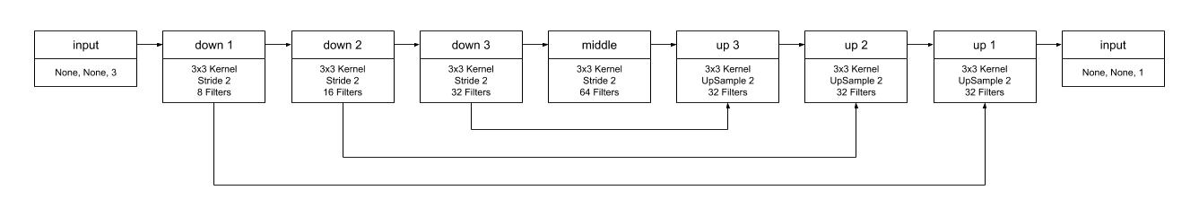
Now that we can generate images to train with, it’s time to start building our model. This is an image translation problem, so a u-net will do nicely.
The basic structure of the network starts with several down convolutional layers, that reduce the image size while adding depth. These are followed by several up layers, up sampling the previous layer applying convolutions, and concatenating the output with the down convolutional output of the same size. Optionally, straight convolutional layers can be added between image resizes for more model depth.
The up layers are concatenated with the down layers to allow the net to easily retain structure present in the original image. This acts similarly to a residual network. It requires the only network to learn how to modify the original image, rather than requiring the network to completely re-build the image.
Here is an basic diagram of the network used, to simplify I have remove the activation, normalization, dropout and concatenation layers. I have also included the code, if you want to take a look.
The results came out great, here are a few random test frames (first row input, middle row correct, last row predicted)
As you can see, it still has a bit of a problem with background noise in some places, but the output is certainly a cleaner indication of where it’s safe to stand.
Now that I have a cleaner input, I need to try feeding that information to my DQN, and see if it helps the RL agent.
Next post: Feeding the detected collision map to a DQN (Blog post coming 5/28/2018)
Special thanks to ◱ PixelyIon for proof reading and other inspiration